Hedging and Trading Strategies

The previous chapter was mainly dedicated to the Black-Scholes model for option pricing. The purpose of this model is not to predict the market movement, but to eliminate risk through hedging. In particular, one can eliminate the instantaneous market risk by constructing a portfolio of an option and the underlying asset with appropriately chosen hedge ratio (Delta). In fact, this can lead to a risk-free portfolio under the model assumptions. The model also provides the price dynamics. A similar idea also appears in the binomial model, where delta hedging is used to replicate the option payoff and derive its price. Thus, pricing and hedging are fundamentally two sides of the same principle.

The concepts used in deriving the pricing models, both in discrete and in continuous time framework, also form the basis for risk management in practice. In particular, delta hedging can be used as a dynamic trading strategy to reduce exposure to movements in the underlying asset. Recall that the delta is defined as the partial derivative of the option price with respect to the underlying asset price \(S\), and hence it measures the sensitivity of the option value to change in \(S\). However, the sensitivity of an option is not limited to the underlying price. One can also analyze the sensitivity of the option value changes with respect to other parameters such as time \(t\), the interest rate \(r\), and volatility \(\sigma\). These sensitivities are commonly represented by Greek letters and they are referred to as Greeks.

In this chapter, we use the pricing framework established in the previous chapters to study how options can be used for risk management and trading. The discussion is organized into two parts. In Section «Click Here», we focus on hedging using sensitivity measures, the Greeks, and examine how these quantities can be used to construct portfolios that reduces exposure to various sources of risk. In Section «Click Here», we turn to commonly used option trading strategies, where options are combined to achieve specific payoff profiles and risk-return characteristics.

Greeks and Hedging

A hedge is a position that offsets the price risk of another position. The main purpose of an option is to hedge a position in an asset. A risk in holding an asset is due to the fluctuations in the underlying asset price, which causes volatility. Thus, the underlying asset price \(S\) and the volatility parameter \(\sigma\) mainly influences an option's price which is also apparent from the Black-Scholes model. It is important to understand the dependency of the option price on \(S\) and \(\sigma\) (also on \(r\) and \(t\)) more closely in order to use options as a powerful hedging tool. To this end, we introduce certain terms that can be used in dependency analysis, called the sensitivity analysis, of the option price on the variables. Some of the sensitivity terms are commonly denoted by Greek alphabets and hence the name Greeks is used in the literature. In this section, we introduce some important Greeks used in option price sensitivity analysis and discuss their usage in hedging strategies.

The Black-Scholes formulae for European put and call options are derived in Corollary «Click Here» and Corollary «Click Here» , respectively. We can see that these prices depend on \(t\), \(S\), \(\sigma\), \(r\), and \(K\). For a fixed strike \(K\), we write the Black-Scholes formulae as

\begin{eqnarray} C(t,S,r,\sigma) &=& S \Phi(d_{+}) - K e^{-r(T-t)}\Phi(d_{-}) ,\\ P(t,S,r,\sigma) &=& K e^{-r(T-t)}\Phi(-d_{-}) - S \Phi(-d_{+}), \end{eqnarray}

(8.1)

where

\[ d_{\pm}(t,S,r,\sigma) = \frac{\log\left(\frac{S}{K}\right)+\left(r\pm \frac{\sigma^2}{2}\right)(T-t)} {\sigma \sqrt{T-t}}. \]

In this section, we analyze the sensitivity of these prices with respect to the parameters \(t\), \(S\), \(\sigma\), and \(r\). More precisely, we study the fundamental properties of the partial derivatives of \(C\) and \(P\) (we use the notation \(V\), the value of an option or a portfolio, in a general discussion not specific to call or put) with respect to the parameters occurring in the Black-Scholes formulae. The collection of all the partial derivatives is called the Greeks. The purpose of studying Greeks is to build hedging portfolios to reduce the sensitivity of the value of a portfolio (or an option) to changes in the underlying by means of diversifying the position.

Delta

Let us start our sensitivity analysis with the dependency of \(V\) with respect to the price of the underlying asset \(S\).

The delta of an option or a portfolio of options is the sensitivity of the option or portfolio to the underlying and is given by

\[ \Delta_V = \frac{\partial V}{\partial S}. \]

We shall now see how the knowledge of delta can be used in hedging a portfolio.

Delta Hedge

Consider the portfolio \(\Pi=(0,\theta,h)\), where \(\theta\) and \(h\) are the number of units in the underlying and the option, respectively.

Then, the value of the portfolio is given by

\[ V = \theta S + hH, \]

where \(S\) is the price of the underlying and \(H\) is the price of the option.

Perfect hedging is to maintain the value \(V\) of the portfolio unchanged while the underlying price fluctuates. This is achieved by selecting \(\theta\) for a given \(h\) (or choosing \(h\) for a given \(\theta\)) such that

\[ \frac{\partial V}{\partial S} = 0. \]

Let \(\Delta_H=\partial H/\partial S\) be the delta of the option. Then, we have

\begin{eqnarray} \theta = -h\Delta_H ~~~\text{or}~~~h = -\frac{\theta}{\Delta_H}. \end{eqnarray}

(8.2)

Note:

Often, give \(h\), finding \(\theta\) is referred to as the delta hedge.

Problem:

Show that

the delta of a European call option is given by
\[ \Delta_C := \frac{\partial C}{\partial S} = \Phi(d_+). \]
the delta of a European put option is given by
\[ \Delta_P := \frac{\partial P}{\partial S} = -\Phi(-d_+). \]

From Problem «Click Here» , we can see that \(\Delta_C>0\) and \(\Delta_P<0\) (the delta for call and put options, respectively). Thus, a short position in call leads to a long spot position and so on.

A portfolio is called delta neutral at some time \(t\in [0,T]\) if \(\Delta_V = 0\) at \(t\).

Building a delta neutral portfolio by having an opposite spot market position in the underlying of an option position is referred to as delta-hedging of a portfolio.

Example:

Consider a \(K\)-strike call (European) option whose delta is given by \(\Delta_C=0.6\). and the lot size is 100. Assume that a trader sold (wrote) 20 call options. Thus, the portfolio of the trader is \(\Pi = (0,\theta,-2000)\) and the value of the portfolio is given by

\[ V = \theta S - 2000\times C. \]

To keep the portfolio delta neutral, we have to choose the number of units of the stock \(\theta\) such that the delta of the portfolio is zero. But the delta of the portfolio is

\[ \Delta_V = \theta - 2000\times 0.6. \]

Thus, in order to keep the portfolio delta neutral (or in order to delta-hedge the portfolio \(\Pi\)) at the present time instance, the trader has to buy \(\theta=1200\) shares in the underlying.

Explanation: At time \(t=0\), let the underlying be trading at ₹ 100 per share and the trader sold the call options at ₹ 10 per share. Then the initial investment in the portfolio \(\Pi\) is

\[ V(\Pi)(0) = 1200\times 100 - 2000 \times 10 = 100000. \]

At time \(t=\Delta t\), let the stock price goes up by ₹ 1.

Since \(\Delta_C=0.6\), we can say approximately that the change in the call option price

\[ C(\Delta t) - C(0) \approx 0.6(S(\Delta t) - S(0)) = 0.6\times 1 = 0.6. \]

Thus, the corresponding call option price is approximately \(C(\Delta t) = 10.6\).

Assuming that the call option price at time \(\Delta t\) is 10.6 per share, the value of the portfolio \(\Pi\) at time \(t=\Delta t\) is given by

\[ V(\Pi)(\Delta t) = 1200\times 101 - 2000\times 10.6 = 100000. \]

Since \(V(\Pi)(0) = V(\Pi)(\Delta t)\), we see that the change in the stock price did not make any profit or loss to the trader leading to a delta neutral portfolio.

Delta drift: Suppose the stock price increases at a later time and consequently the call delta also increased to, say \(\Delta_C = 0.7\). Since the hedge position remains \(\theta=1200\), the portfolio delta is no longer zero and is given by

\[ \Delta_V = -200, \]

which is the delta drift of the portfolio caused by the price changes.

Remark:

Delta hedging is based on a first-order approximation and is therefore accurate over a very short time period, i.e. when \(\Delta t\) is very small, and when the stock price variation is very small. If the time step is large or the stock price variation is very large, then one has to recompute the delta of the option (\(\Delta_C\) or \(\Delta_P\) depending on whether the traded option is a call or a put option, respectively) and reconstruct the delta-hedging portfolio. This process is called the rebalancing of the portfolio.

If a hedged position is rebalanced time to time to maintain a delta-neutral portfolio, then the hedging process is called the dynamic hedge. On the other hand, if a hedging position is held over time without rebalancing, then the hedging process is called the static hedge.

In the following example, we illustrate the dynamic hedging to maintain a delta-neutrality of a portfolio. The aim is also to show that we can maintain delta-neutrality not only by trading in the underlying asset but also by adjusting positions in multiple options. In particular, we consider a portfolio of two call options and show the procedure for achieving the delta neutrality by trading the underlying asset or by modifying the option positions.

Example:

Consider two call options on the same underlying asset and expiration \(T\):

\(K_1=22,150\) with premium \(C_{1,0}=89\);
\(K_2=22,250\) with premium \(C_{2,0}=48\).

Here, we used the notation \(C_{1,0}\) for \(C_1(t_0)\) and a similar notation for the other option.

Consider a portfolio \(\Pi = (0,\theta, (c_1, -c_2))\). Here, \(\theta\) is the number of units in the underlying, and \(c_i > 0\), \(i=1,2,\) is the number of units held in the \(K_i\)-strike call option.

Consider the portfolio at time \(t=t_0\) as \(\Pi_1 = (0,0, (c, -c))\), for some c > 0. Such a portfolio is called a bull spread. A more detailed discussions on bull spread and similar other trading strategies are discussed in the next section.

At time \(t_0 < t_1 < T\), assume that the price of \(K_1\)-strike option is \(C_{1,1} = 155\) with delta \(\Delta_{1,1}=0.53\) and \(K_2\)-strike price is \(C_{2,1}=65\) with delta \(\Delta_{2,1}=0.44.\).

Our interest is to adjust the portfolio \(\Pi_1\) at time \(t=t_1\) to obtain a delta-neutral portfolio. There are two ways to achieve this.

Method 1: Delta Hedging

Delta neutrality can be achieved through delta-hedging, where an appropriate position is taken in the underlying asset, whereas the option positions are kept unchanged. Let the new portfolio be \(\Pi_2 = (0,\theta, (c, -c))\).

In this case we have to find \(\theta\) such that \(\Delta_V=0\). Thus, we have

\[ \theta = -c(\Delta_{1,1} - \Delta_{2,1}) = -0.09c. \]

Therefore, the delta-hedge portfolio adds a short position in the underlying asset, which offsets the positive delta of the option portfolio.

Method 2: Option Rebalancing or Adjustment Using Options

We have \(\Pi_1 = (0,0,(1,-1))\) created at time \(t=t_0\). At time \(t=t_1\), we have to make another portfolio \(\Pi_2\) such that \(\Delta_{V_2} = 0\). Let the portfolio be \(\Pi_2 = (0,0,(c,-c_2))\). Then, we have

\[ V_1(\Pi_2) = c C_{1,1} - c_2C_{2,1}. \]

Therefore, \(\Delta_{V}=0\) implies

\[ c_2 = \frac{\Delta_{1,1}}{\Delta_{2,1}} c \approx 1.2045 c. \]

We already hold \(c\) units of \(K_2\)-strike option in our portfolio. Therefore, we must short an additional \(c_2 - c = 0.2045 c\) units of \(K_2\)-strike option to make the portfolio \(\Pi_2\).

Note:

The portfolio adjustment illustrated in the above example is only one way to achieve a delta-neutral position. In general, delta neutrality is not unique. For instance, we may also adjust the position in the \(K_1\)-strike option, or use other traded options (example, a \(K_3\)-strike option) possibly with a different expiration. The choice of instruments typically depends on market liquidity and trading considerations.

Problem:

As a continuation of the above example, consider a scenario at time \(t=t_2\) with \(t_0 < t_1 < t_2 < T\) as \(C_{1,2}=237\), \(C_{2,2}=129\), \(\Delta_{1,2}=0.5\) and \(\Delta_{2,2}=0.32\).

Assume that at time \(t_1\) the portfolio is \(\Pi_2 = (0, 0, (c, -c_2))\).

Obtain a delta-neutral portfolio \(\Pi_3\) by hedging \(\Pi_2\) (this means we have to make changes in the underlying asset).
Alternatively, obtain \(\Pi_3\) by adjusting the position in the \(K_2\)-strike option (while keeping the position in the \(K_1\)-strike option fixed) to achieve a delta neutral portfolio at time \(t_2\).

From the above example and problem, we obtain a three level dynamic delta-neutral portfolio strategy \(\{\Pi_1, \Pi_2, \Pi_3\}\). We can extend this procedure to any number of time steps. Theoretically, we can even obtain a continuous time delta-neutral portfolio strategy \(\{\Pi_t\}\), which is naturally modelled as a stochastic process and forms the basis of the Black-Scholes framework.

Remark:

[Dynamic Delta-Hedging Strategy]

Let the initial portfolio \(\Pi_1\) be set at time \(t=0\) (this may or may not be delta-neutral).

As time evolves and the underlying asset price changes, the deltas of the options also change. In order to maintain delta-neutrality, we have to adjust the portfolios time-to-time.

To this end, let us consider a discrete time levels \(0=t_0 < t_1 < \ldots < t_n = T\) at which we adjust the portfolio to restore delta-neutrality.

As illustrated in the above example, delta-neutrality can be achieved in multiple ways. In particular, adjusting the position in the underlying asset wile keeping the option positions unchanged, is referred to as a delta-hedging strategy. Since delta-hedging is carried out at each time level, the process \(\{\Pi_1, \Pi_2, \ldots, \Pi_n\}\) is often referred to as the dynamic delta-hedging strategy.

Note:

A dynamic hedging strategy can also be made a self-financing strategy by making the risk-free component non-zero.

Gamma

In the previous subsection, we developed the idea of delta hedging and discussed how a portfolio can be made locally insensitive to small changes in the underlying asset price by maintaining delta-neutrality. This was achieved through dynamic rebalancing of the portfolio at discrete time points.

Since delta hedging is based on the first-order approximation of the option price

\[ dC \approx \Delta\, dS. \]

a delta-neutral portfolio eliminates only the first-order sensitivity to changes in the underlying price. However, in practice, the option price depends nonlinearly on the underlying asset price and consequently, the delta-neutral portfolio is exposed to residual risk.

There are two ways to reduce this residual risk. One way is to rebalance the portfolio more frequently. Another approach is to improve the accuracy of the hedge by incorporating gamma into the hedging strategy, which is defined for a portfolio as

\[ \Gamma = \frac{\partial^2 V}{\partial S^2}. \]

A more accurate approximation involving gamma is given by

\[ dC \approx \Delta\, dS + \tfrac{1}{2}\Gamma (dS)^2, \]

and the delta-neutral portfolio using the above approximation is now exposed to a second-order residual risk.

Gamma measures the curvature of the option price with respect to the underlying asset price, or equivalently, the rate of change of delta with respect to the underlying price.

The gamma of an European call and put options are defined similarly and are denoted by \(\Gamma_C\) and \(\Gamma_P\), respectively.

Problem:

Using Black-Scholes formula for European call options show that

\[ \Gamma_C = \frac{e^{-\frac{d_{+}^2}{2}}}{\sqrt{2\pi(T-t)}S\sigma}. \]

Use put-call parity relation to obtain the expression for the European put option gamma \(\Gamma_P\).

We now illustrate the construction a delta-gamma hedging portfolio that is insensitive to both first- and second-order changes in the underlying asset price.

Example:

Consider a European call options with two strikes, \(K_1\) and \(K_2\), with prices denoted by \(C_1\) and \(C_2\), respectively. The portfolio is given by \(\Pi=(0,\theta,\boldsymbol{c})\), where \(\boldsymbol{c}=(c_1,c_2)\) is the vector with components being the number of units in the respective options. The value of the portfolio is given by

\[ V = \theta S + c_1C_1 + c_2C_2. \]

Differentiating with respect to \(S\) twice, we get

\[ \Delta_V = \frac{\partial V}{\partial S} = \theta + c_1\Delta_{C_1} + c_2\Delta_{C_2} \]

and

\[ \Gamma_V = \frac{\partial^2 V}{\partial S^2} = c_1\Gamma_{C_1} + c_2\Gamma_{C_2}. \]

Equating both the above expressions to zero, we get the linear system

\[ \begin{array}{c} \theta + c_1\Delta_{C_1} + c_2\Delta_{C_2}=0\\ c_1\Gamma_{C_1} + c_2\Gamma_{C_2}=0. \end{array} \]

Given the values of \(\Delta_{C_j}\) and \(\Gamma_{C_j}\), \(j=1,2\), and fixing one of the variables \(\theta\) and \(c_j\), \(j=1,2\), the above system can be solved (if possible) to obtain the delta-gamma-hedging portfolio.

Interpretation: One of the options is used to neutralize gamma, while the position in the underlying asset is then adjusted to eliminate the remaining delta.

Note:

Since \(\Gamma_{C_j}\), \(j=1,2\), are positive, we need one of \(c_1\) and \(c_2\) to be negative in the above system to have a nonzero solution for the second equation. Hence one needs to take opposite positions in the two call options in order to obtain a delta-gamma-hedging porfolio.

Problem:

[Delta-Gamma Hedging with Call and Put]

Consider a European call option \(C_1\) with strike \(K_1\) and a European put option \(P_2\) with strike \(K_2\), both written on the same underlying asset with the same maturity \(T\).

At a given time \(t\), suppose:

\[ \begin{array}{c} \Delta_{C_1} = 0.60, \quad \Gamma_{C_1} = 0.020,\\ \Delta_{P_2} = -0.35, \quad \Gamma_{P_2} = 0.015. \end{array} \]

Consider a portfolio of the form

\[ \Pi = (0,\theta, \boldsymbol{h}), \]

where \(\theta\) is the number of units of the underlying asset, and \(\boldsymbol{h} = (c, p)\) with \(c\) and \(p\) being the number of units of the call and put options, respectively.

Find the relation between \(c\) and \(p\) required for gamma-neutrality.
Express \(\theta\) in terms of \(c\) so that the portfolio is delta-neutral.
If \(c = 100\), determine \(p\) and \(\theta\).

Answer: (3) \(p\approx -133.33\), \(\theta\approx -106.67.\)

Theta

So far we have seen that delta and gamma measure the sensitivity of the option price with respect to the underlying asset. As the option price depends on time, it is also important to include time sensitivity in hedging, which is known as theta, and is defined for a portfolio of options as

\[ \Theta = \frac{\partial V}{\partial t}. \]

The theta of European call and put options is defined similarly and is denoted by \(\Theta_C\) and \(\Theta_P\), respectively.

Problem:

Using Black-Scholes formula for European \(K\)-strike call option show that

\[ \Theta_C = -\frac{S\sigma}{2\sqrt{2\pi(T-t)}} e^{-\frac{d_{+}^2}{2}} - rKe^{-r(T-t)}\Phi(d_-). \]

Using call theta expression and without differentiating the Black-Scholes formula for put option (rather using put-call parity relation), show that the theta of the corresponding put option is given by

\[ \Theta_P = -\frac{S\sigma}{2\sqrt{2\pi (T-t)}} e^{-d_+^2/2} + r K e^{-r(T-t)} \Phi(-d_-). \]

We have seen that a delta-gamma neutral portfolio eliminates the second-order sensitivity to changes in the underlying asset. Using a second-order Taylor expansion, the change in the value of a portfolio \(V(t,S)\) is given by

\[ dV \approx \Theta_V\, dt + \Delta_V\, dS + \tfrac{1}{2}\Gamma_V (dS)^2. \]

For a delta-gamma neutral portfolio (i.e., \(\Delta = 0\) and \(\Gamma = 0\)), this reduces to

\[ dV \approx \Theta\, dt. \]

Thus, a delta-gamma neutral portfolio is still exposed to changes in value arising from time decay.

Since the value \(V=V(t,S)\) of a portfolio of options (with the same underlying) satisfy the Black-Schole PDE (7.20), the theta of \(V\) is given by

\[ \Theta_V = -\frac{1}{2}\sigma^2 S^2 \Gamma_V - r S \Delta_V + r V. \]

For simplicity, let us assume that the portfolio is delta neutral. Then, we have

\[ \Theta_V = -\frac{1}{2}\sigma^2 S^2 \Gamma_V + r V. \]

From this expression, we see that if \(\Gamma_V>0\), then as it increases, \(\Theta_V\) becomes negative and tends to decrease. This increases the magnitude of time decay. Thus, if the graph of the portfolio value in terms of \(S\) is convex, then the portfolio typically experiences time decay.

On the other hand, if \(\Gamma_V<0\), then \(\Theta_V\) tends to be positive, and the portfolio benefits from the passage of time.

Note:

Theta measures the sensitivity of the portfolio value to the passage of time. Theta cannot be directly hedged, however, it plays an important role in risk management and reflects the cost (or benefit) of holding a given exposure to convexity.

Vega

The vega of an option or a portfolio of options is defined as

\[ \mathcal{V} = \frac{\partial V}{\partial \sigma}, \]

where \(\sigma\) denotes the volatility parameter in the Black-Scholes model. Vega measures the sensitivity of the option value to changes in volatility, and in practice is interpreted with respect to changes in implied volatility.

The vega of a European call and put options are defined similarly and are denoted by \(\mathcal{V}_C\) and \(\mathcal{V}_P\), respectively.

For standard European options, vega is positive, reflecting the fact that option values increase with volatility.

Problem:

Using Black-Scholes formula for European call option show that

\[ \mathcal{V}_C = \frac{S\sqrt{T-t}}{\sqrt{2\pi}} e^{-\frac{d_{+}^2}{2}}. \]

Is the vega of call and put option under the Black-Scholes formula are same? Justify your answer.

To hedge against the underlying volatility, one can construct a vega-hedging by equating \(\mathcal{V}=0\). Unlike delta hedging, this typically requires two option positions in the portfolio to have vega hedge as the hedging cannot be achieved using the underlying asset because \(\frac{\partial S}{\partial \sigma} = 0\).

Example:

Consider a portfolio \(\Pi = (0,\theta, \boldsymbol{h})\), where \(\boldsymbol{h} = (c, p).\) Then, we have

\[ V = \theta S + c C + p P. \]

The portfolio vega is given by

\[ \mathcal{V}_V = \theta \frac{\partial S}{\partial \sigma} + c \mathcal{V}_C + p \mathcal{V}_P. \]

For vega neutral portfolio, we need to choose \(c\), for a given \(p\) (or equivalently choose \(p\) for a given \(c\)), such that \(\mathcal{V}_V = 0\). That is

\[ c = -p\frac{\mathcal{V}_P}{\mathcal{V}_C}. \]

One can also perform delta-vega and gamma-vega hedging in a similar way as in the case of delta-gamma hedging. By including multiple options on the same underlying asset (with possibly different strikes and/or maturities) together with the underlying itself, one can construct portfolios that are simultaneously neutral with respect to delta, gamma, and vega. The minimum number of instruments required follows from the number of constraints imposed.

Rho

The rho of an option or a portfolio of options is defined as

\[ \rho = \frac{\partial V}{\partial r} \]

The rho of a European call and put options are defined similarly and are denoted by \(\rho_C\) and \(\rho_P\), respectively.

Problem:

Using Black-Scholes formula for European \(K\)-strike call option show that

\[ \rho_C = (T-t)Ke^{-r(T-t)}\Phi(d_-). \]

Also, obtain the expression for \(\rho_P\).

Note:

In many practical settings, particularly for short-dated equity options, rho plays a relatively minor role compared to other Greeks such as delta, gamma, and vega. However, it becomes significant for long-dated options and in interest-rate-sensitive markets.

Option Trading Strategies

There are many strategies to make portfolios by combining options and the underlying assets. One can also build portfolios by combining several options. We discuss here a few which are more popular.

Options are primarily used for hedging. However, speculators come into the market as a consequence of high liquidity. Speculators are also attracted to a great advantage of leverage in trading options rather than trading directly in the underlying assets. The idea of leverage is well understood through simple examples.

Example:

[Leverage]

Assume that a stock traded at the spot market for ₹ 1950 per share on 1\(^{\rm st}\) February and the same stock was trading at ₹ 2150 on 25\(^{\rm th}\) February. Mr. Megh bought 100 shares of the stock on 1\(^{\rm st}\) February by paying ₹ 1,95,000 and sold it on 25\(^{\rm th}\) February and obtained ₹ 20,000, which gave him 10.26% on his initial investment.

On the other hand, Mrs. Sahana bought a call option (with contract size 100 shares) for 1950-strike, expiration 25\(^{\rm th}\) February, and the premium of ₹ 50 per share. Hence, she paid ₹ 5000 (= \(X\)) as the premium to the call option. On the expiration date, the spot price was \(S_T = 2150\). Since the strike price was less than the spot price of the stock at expiration, Mrs. Sahana's call option was in-the-money. So, she would certainly exercise the option on the expiration and gone for the cash settlement of

\[ C_T = (2150-1950)\times 100 = 20,000 ~(\text{payoff}). \]

Since she paid 5000 as premium, the gain in the trade (with \(r=0\)) was

\[ G_T = 20000 - 5000 = 15,000. \]

Mrs. Sahana obtained ₹ 5000 less than Mr. Megh's return in the spot market trade. However, Mrs. Sahana's gain was 300% of her initial investment, whereas Mr. Megh obtained only 10.26%.

Obtaining a higher percentage return from an option is called leverage. In other words, the call option that Mrs. Sahana opted for had provided a leveraged return to her.

Caution: On the contrary to the scenario considered above, if the spot price of the stock on 25\(^{\rm th}\) February was at ₹ 1949, say, just ₹ 1 less than the strike price. Then, compute the percentage loss for Mrs. Sahana and Mr. Megh.

In the above example, the options trader is a speculator. This is because the trader's intention was not to reduce the uncertainty in the price fluctuation of a stock in the portfolio. Instead, the trader somehow predicted that the stock price would go up (or merely guessed it) and took a risk in the trade.

Hedgers are just opposite to speculators. They are more worried about the risk involved in their investment, and they do not mind compromising some portion of their return to reduce the risk. This is something similar to insurance. A hedge can be understood through simple examples.

Protective put graph for Example «Click Here» .

Example:

[Hedge using protective put]

Assume that Mr. Megh bought 100 shares of a stock at the rate of ₹ 1950 per share on 1\(^{\rm st}\) February. He anticipated an up move in the stock price by the end of February, and hence he had the intention of selling it by the month-end. However, he was worried about the possibility of the stock price going downwards. He decided to reduce his risk by looking for an option.

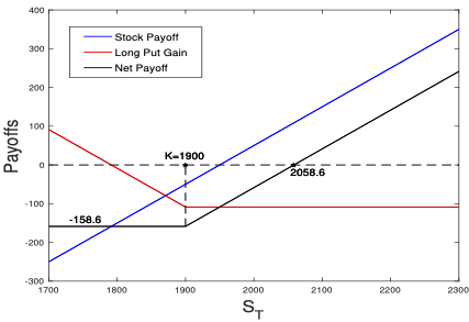
Mr. Megh noticed a put option with 1900-strike, expiration 25\(^{\rm th}\) February, and the premium of ₹ 108.6 per share. He took a long position in one put option, whose contract size ( i.e. lot) was 100 shares.

Mr. Megh's long put trade gave him a downward protection, which can be seen from the net gain given by

\begin{eqnarray} \mathcal{N}(S_T) &=& \text{Stock payoff} + \text{Long put gain/loss}\\ &=& (S_T - S_0) + G_T, \end{eqnarray}

(8.3)

where \(S_0=1950\) and \(G_T\) is calculated with \(r=0\).

Figure «Click Here» depicts the payoff graph.

One can see that the long put option position limited Mr. Megh's loss (which we call limited loss) in the spot market trade to \(-158.6\) per share, and the profit is unbounded. One can also see that Mr. Megh makes a profit if \(S_T>2058.6 =:S_*\).

Protecting a risky investment from losing too much using some counter trades (in the present case, it is the long put) is a hedge. In other words, the put option Mr. Megh opted for had provided a hedge for his exposure to the stock that he traded in the spot market.

Problem:

[Hedge using covered call]

Obtain a hedge for Mr. Megh in the above example using the following call option:

1990-strike;

expiration 25\(^{\rm th}\) February;

contract size 100; and

premium ₹ 91 per share. Obtain the net gain function, limited loss, and the minimum stock price \(S_*\) such that \(S_T>S_*\) gives profit to Mr. Megh. Also, draw the graphs of stock payoff, gain/loss of the call, and net gain.

Hint:

See whether you have to enter into the call option trade as a writer or a holder. In other words, see whether you have to take a short or a long position in the call option in order to hedge the spot market trade. For the net gain function, give the complete expression, including the expression for gain/loss; just writing \(G_T\) is not enough.

Remark:

[Covered put]

A covered put is a portfolio involving a short position in the spot market and a short position in the corresponding option.

Spreads

A spread is a portfolio consisting of options of the same type (either all calls or all puts). There are three basic kinds of spreads:

A vertical spread (or price spread) is a portfolio in which the options have the same expiration date but different strike prices.
An horizontal spread (or calendar spread) is a portfolio in which the options have the same strike price but different expiration dates.
A diagonal spread is a portfolio in which the options have different strike prices and expiration dates.

We restrict to only vertical spreads and discuss some popular vertical spreads among traders.

Bull Spread

Bull spread is a portfolio created when a trader anticipates an upward trend in the underlying asset price.

Definition:

For given \(0 < K_1 < K_2\), the portfolio consisting of a long position in a \(K_1\)-strike call (put) option and a short position in a \(K_2\)-strike call (put) option with the same expiration and the same underlying asset is called a bull spread.

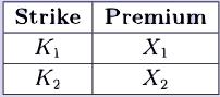
A bull spread is an example of a vertical spread. The general form of the net gain function for bull spread is given by

\begin{eqnarray} \mathcal{N}(S_T) &=& \text{Gain in Long call}~ + \text{Gain in Short call}\\ &=&\big(\max(0,S_T-K_1) - X_1\big)+\big(X_2-\max(0,S_T-K_2)\big)\\ &=&\left\{\begin{array}{ll} X_2-X_1,&\text{if } S_T\le K_1\\ S_T-K_1 + X_2-X_1,&\text{if } K_1\le S_T\le K_2\\ K_2-K_1 + X_2-X_1,&\text{if } K_2\le S_T. \end{array}\right. \end{eqnarray}

(8.4)

Observe that in order to maximize the profit, we have to look for maximizing \(K_2-K_1\) and minimize \(X_2-X_1\), wherever the later is negative. Note that \(X_2-X_1\) is typically negative in practice. Opting for out-of-the-money calls, which generally trade with lower premiums, can be advantageous in this regard.

Gain graphs for Example «Click Here» .

Example:

Mrs. Sahana believes that the share price of a stock will increase to ₹ 2150 in a month from its current price of ₹ 1950. In other words, Mrs. Sahana is bullish on the stock. She can perform one of the following trades:

she can buy the stock at the spot market; or

she can buy a future in the futures market; or

she can buy a 1950-strike call option; or

she can write a 1950-strike put option. The first choice is expensive, and all the choices are highly risky. However, if her prediction goes correct, they all will give a considerable profit.

Alternatively, Mrs. Sahana can go for a bull spread if she is ready to give up a part of the predicted profit.

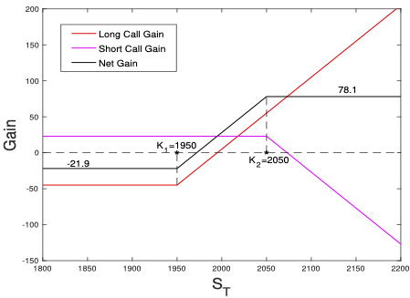
Mrs. Sahana made the following portfolio 1\(^{\rm st}\) February:

She bought the 1950-strike European call option for the premium ₹ 44.90 per share; and

sold the 2050-strike European call option for the premium ₹ 23 per share, both have expiration 25\(^{\rm th}\) February. From the above description, we can see that the above trades give rise to a portfolio, which is a bull spread.

The net gain of the bull spread is given by

\begin{eqnarray} \mathcal{N}(S_T) = \left\{\begin{array}{ll} -21.9,&\text{if } S_T\le 1950\\ S_T-1971.9,&\text{if } 1950\le S_T\le 2050\\ 78.1,&\text{if } 2050\le S_T. \end{array}\right. \end{eqnarray}

(8.5)

The gain graphs are depicted in Figure «Click Here» . Observe that Mrs. Sahana had invested ₹ 21.9 per share. The maximum loss that she can take in this portfolio is \(-21.9,\) and the maximum profit she can achieve is 78.1.

Problem:

Consider the following active call options trading at the market and all these options have the same expiration:

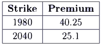
Construct a bull spread out of these call options. Obtain the general form of the net gain function and also obtain the net gain function for this problem. Draw the gain graphs for all the traded options and also draw the graph of the net gain function.

Note:

One can also create a bull spread with put options.

Problem:

Consider two active European put options

trading at the market with same underlying and expiration with \(K_1. Construct a bull spread out of these put options and obtain the general form of the net gain function. In particular, if \(K_1=1500\), \(X_1=30.05\), \(K_2=1520\), and \(X_2=40.45\), then obtain the net gain function for the bull spread. Draw the gain graphs for all the traded options and also draw the graph of the net gain function.

Bear Spread

Bear spread is a portfolio formed by a trading having a bearish view on the underlying asset price.

Definition:

[Bear Spread]

For given \(0 < K_1 < K_2\), a bear spread is a portfolio can be created by buying a \(K_2\)-strike call (put) option and write a \(K_1\)-strike call (put) option with the same underlying asset and a same expiration date.

Problem:

Obtain the general form of the net gain function of the following:

a bear call spread
a bear put spread

Example:

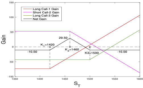
On 2\(^{\rm nd}\) March 2020, Mrs. Sahana felt that the entire market would crash in a month. In particular, she felt that HDFC Bank stock, which was trading at ₹ 1200 per share on the day, would crash up to ₹ 1100 per share. In other words, Mrs. Sahana was bearish on the HDFC Bank's stock.

Mrs. Sahana constructed a bear spread out of the stock options as follows:

she bought a European put option of 1180-strike with premium ₹ 28; and

she wrote another European put option of 1140-strike with premium ₹ 20,

both had expiration 28\(^{\rm th}\) March 2020.

The net gain of the bear spread is given by

\begin{eqnarray} \mathcal{N}(S_T) = \left\{\begin{array}{ll} 32,&\text{if } S_T\le 1140\\ 1172 - S_T,&\text{if } 1140\le S_T\le 1180\\ -8,&\text{if } 1180\le S_T. \end{array}\right. \end{eqnarray}

(8.6)

The gain graphs are depicted in Figure «Click Here» . Observe that Mrs. Sahana had invested ₹ 8 per share to build the portfilio. The maximum loss that she can take in this portfolio is \(-8,\) and the maximum profit she can achieve is 32.

Gain graphs for Example «Click Here» .

Note:

One can also create a bear spread with call options.

Problem:

The following are the active put options trading at the market on 2\(^{\rm nd}\) March 2020:

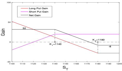
Mrs. Sahana (in Example «Click Here» ) is looking for another bear spread. All the options were with expiration 28\(^{\rm th}\) March 2020. Suggest another bear spread than the one opted in Example «Click Here» . Obtain the net gain per share and draw the gain graphs.

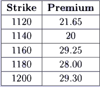
Butterfly Spread

Definition:

Let \(0 < K_1 < K_2 < K_3\), and \(K_2\in [S_0-\epsilon,S_0+\epsilon]\) for some sufficiently small \(\epsilon > 0\). Buy two call options, one in each of \(K_1\)-strike and \(K_3\)-strike. Write two call options with \(K_2\)-strike. All options have the same underlying and expiration. The resulting portfolio is a butterfly spread.

Note:

The role of \(\epsilon\) in the above definition is to indicate that \(K_2\)-strike option is very near to the in-the-money option. It is not always necessary that \(\epsilon\ll 1\). Practically, \(K_2\) can be \(\pm 1%\) of the spot price or even more depending on the situations.

The general form of the net gain function for butterfly spread is given by

\begin{eqnarray} \mathcal{N}(S_T) &=& \text{Gain in Long call-1} + 2\times \text{Gain in Short call-2} + \text{Gain in Long call-3}\\ &=&\big(\max(0,S_T-K_1) - X_1\big)+2\big(X_2-\max(0,S_T-K_2)\big) \\ &&~~~~~~~~~~~~~~+\big(\max(0,S_T-K_3) - X_3\big)\\ &=&\left\{\begin{array}{ll} -X_1+2X_2-X_3,&\text{if } S_T\le K_1\\ S_T-K_1-X_1+2X_2-X_3,&\text{if } K_1\le S_T\le K_2\\ -S_T-K_1+2(K_2 + X_2)-X_1-X_3,&\text{if } K_2\le S_T\le K_3\\ -K_1+2K_2-K_3-X_1 + 2X_2-X_3,&\text{if } K_3\le S_T. \end{array}\right. \end{eqnarray}

(8.7)

Example:

Assume that Titan was trading at ₹ 1457 (\(=S_0\)) per share on 1\(^{\rm st}\) February 2021. Mrs. Sahana felt that the share price would not vary significantly during the month. Based on her prediction, she made the following trades:

she wrote two call options with 1460-strike at the premium of ₹ 52.7 per share;

she bought one call option with 1420-strike for ₹ 73.2 per share; and

she also bought one call option with 1500-strike for ₹ 42.7 per share. With these trades, she created a portfolio which is a butterfly spread.

The net gain of the butterfly spread is given by

\begin{eqnarray} \mathcal{N}(S_T) = \left\{\begin{array}{ll} -10.5,&\text{if } S_T\le 1420\\ S_T-1430.5,&\text{if } 1420\le S_T\le 1460\\ 1489.5-S_T,&\text{if } 1460\le S_T\le 1500\\ -10.5,&\text{if } 1500\le S_T. \end{array}\right. \end{eqnarray}

(8.8)

The gain graphs are depicted in Figure «Click Here» .

Gain graphs for Example «Click Here» .

Note:

One can also create a butterfly spread with put options.

Problem:

The following are the active call options trading at the market on 1\(^{\rm st}\) February 2021, and Mrs. Sahana (in Example «Click Here» ) is looking for a better butterfly spread:

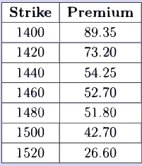
All the options are with expiration 25\(^{\rm th}\) February 2020. Suggest a butterfly spread different from the one opted in Example «Click Here» . Obtain the net gain per share and draw the gain graphs. Also, write the portfolio and find its initial value using the mathematical notations introduced in the course.

Problem:

Consider the following active put options trading at the market and all these options have the same expiration :

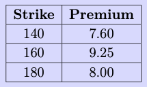
The current spot market price of the underlying stock is ₹ 160.2. Construct a butterfly spread out of these put options. Obtain the general form of the net gain function and also obtain the net gain function for this problem. Draw the gain graphs for all the traded options and also draw the graph of the net gain function.

Volatility Speculation

The bull and bear spreads are directional speculations, whereas the butterfly spread is a volatility speculation. In this section, we introduce two more strategies used as volatility speculations.

Straddle

A straddle is a portfolio made by taking long positions in a call and a put simultaneously with the same strike price, underlying asset, and the expiration.

For a given \(K>0\), the general form of the net gain function of a straddle is given by

\begin{eqnarray} \mathcal{N}(S_T) &=& \text{Gain in Long call} + \text{Gain in Long put}\\ &=&\big(\max(0,S_T-K) - C\big)+\big(\max(0,K-S_T) - P\big)\\ &=&\left\{\begin{array}{ll} -S_T+K-C-P,&\text{if } S_T\le K\\ S_T-K-C-P,&\text{if } K\le S_T. \end{array}\right. \end{eqnarray}

(8.9)

A trader anticipating a less volatility in the underlying asset can take a short straddle, means that the trader should take short positions in both options. On the other hand, if a trader thinks that the stock price will be volatile, but not clear about which direction it will move, then a (long) straddle may be preferred.

Strangle

The disadvantage of straddle is that both the options have the same strike price. Thus, we have to go for either both at-the-money options or one in-the-money and another out-of-the-money options. In any case, we can see that the total price of the portfolio will be high. Generally, out-of-the-money options are cheaper than in-the-money options. Therefore, if we relax the condition of having the same strike price, we can building portfolio with two long positions, one in call and another in put, but now with different strike prices. Such a portfolio is called a strangle.

For given real numbers \(0 < K_1 < K_2\), a portfolio consisting of a long \(K_1\)-strike put option and a long \(K_2\) strike call option on the same underlying and with same expiration is called a strangle (also called long strangle). A short strangle is a short position in a strangle, which means selling a \(K_1\)-strike put option and a \(K_2\) strike call option on the same underlying and with same expiration.

Problem:

Determine the net gain function for both a long strangle and a short strangle.

Given a pair of real numbers \(0 < K_1 < K_2\), find the positive real numbers \(S_*\) and \(S^*\) such that the net gain function in the corresponding (long) strangle satisfies:

\[ \mathcal{N}(S_T) > 0, \text{ for all } S_T < S_* \text{ and } S_T > S^*. \]